
Neural Networks and Deep Learning: How Machines Actually Learn
Data Science Journey 2026 — Step 7
In the last article, we built the first real machine learning model, a Decision Tree Classifier on the Iris Dataset, and watched it hit around 96% accuracy identifying flower species, just by asking the right yes/no questions.
Every AI system you’ve heard of, like image recognition, recommender systems, ChatGPT, self-driving cars, all of it is based on “Neural Networks”.
By the end of this post, you won’t just know what a neural network is; you’ll understand how one is built, trained, and how it learns to read handwritten digits, in plain terms.
Why a Decision Tree Isn’t Enough Anymore?
In Step 6, our Decision Tree worked because Iris dataset have a handful of clean, structured measurements: Petal Length, Petal Width, Sepal Length and Sepal Width and a good yes/no question like “is Petal Length under 2.45?” cleanly separates them.
Now imagine a new task: look at the image below and tell me if it’s a 4 or a 9?
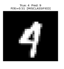
An image like this does not contain measurements; it’s 784 numbers, one for every pixel in a 28×28 grid. What yes/no question could you possibly write? “Is pixel number 400 dark ?” That tells you almost nothing on its own. The pattern that makes a 4 a 4 isn’t in any single pixel, but it’s how hundreds of pixels relate to each other at once.
This is exactly the kind of problem Machine Learning Algorithms struggle with, and exactly the kind of problem neural networks were built for.
What Is a Neural Network, Really?
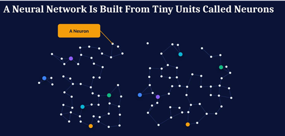
A neural network is built from tiny units called ‘neurons’. Each neuron does something almost embarrassingly simple: it takes in some numbers, multiplies each one by a ‘weight‘ (a number that says how important that input is), adds them all up, adds one more adjustable number called a ‘bias‘, and passes the result through a small function that decides how strongly to “fire.”
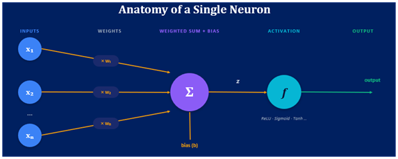
A single neuron, structurally: inputs → weights → weighted sum + bias → activation function → output as shown in the above image.
Think of a single neuron like a tiny voter looking at evidence. It doesn’t decide anything on its own, but it casts a weighted opinion. Stack enough of these voters together, in layers, and something remarkable happens: the network as a whole can learn to recognize patterns far too complex for any single yes/no rule.
That’s the “magic”: weighted votes, stacked in layers, adjusted until they get good at a task.
The Anatomy of a Network
Here’s the architecture we’re going to build for our digit image.
Input Layer (784) → Hidden Layer(s) → Output Layer (10).
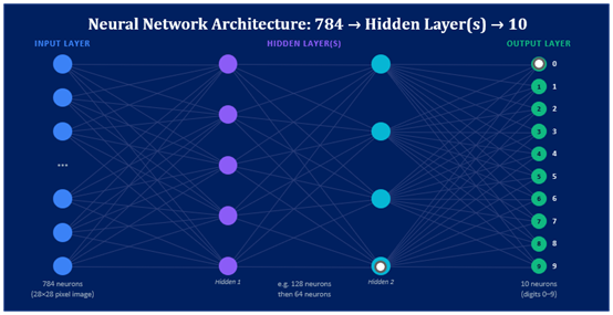
An Input Layer
The input layer is one neuron for every pixel in our image, so 784 of them, just passing in the raw data.
Hidden Layers
One or more Hidden Layers; this is where the real pattern-detection happens. Early neurons might learn to notice edges or curves; later ones combine those into loops, lines, and corners makes the building blocks of a digit.
Output Layer
An Output Layer consists of 10 neurons, one for each digit, 0 through 9. Whichever one fires the strongest is the network’s guess.
And here’s where the word “deep” comes from in Deep Learning; it simply means a network with several hidden layers stacked on top of each other, each one learning slightly more complex patterns than the last.
The Learning Loop: How It Actually Learns
Here’s the part everyone wants to understand: how does a neural network actually learn?
The four steps, repeated thousands and thousands of times:
Forward Pass → Loss → Backpropagation → Adjust Weights → repeat.
1. Forward Pass
The network takes an image and makes a guess. For now, a bad one, since every weight starts randomly.
2. Loss
It compares that guess to the real answer and calculates a number that says exactly how wrong it was. This is called the loss.
3. Backpropagation
This is the clever part. The network sends that error signal backward, layer by layer, working out exactly how much each weight contributed to the mistake.
4. Gradient Descent(Optimizer)
Here, every weight gets nudged, just slightly, in the direction that would have reduced the error.
Then it repeats. On the next image. And the next. Thousands of times per second, across an entire dataset, again and again, across what we call ‘epochs’. There’s no understanding, no intuition, just relentless, mechanical trial, error, and tiny correction, at a scale and speed no human could ever do by hand. That is, quite literally, how machines learn.
Implementing a Neural Network on the MNIST Dataset
We hit a wall a Machine Learning Algorithm couldn’t cross, recognizing handwritten digits from raw pixels, and met the tool built for exactly that: the neural network. We broke a single neuron down into weights, bias, and activation. We stacked neurons into input, hidden, and output layers, and understood what “deep” actually means. We walked through the four-step learning loop: forward pass, loss, backpropagation, gradient descent.
We will build a real one in TensorFlow and Keras, train it on 60,000 handwritten digits of the MNIST Dataset, and watch it reach roughly 97–98% accuracy on images it had never seen.
Download Complete Jupyter Notebook
Download the complete Jupyter Notebook on Neural Networks and Deep Learning by clicking on the link below:
Stay Tuned!!
Congratulations! You have just learned and built your first Neural Network on the MNIST dataset.
Explore the complete Data Science Series with article links, Jupyter notebooks, and YouTube links mentioned below:
Keep learning and keep implementing!!


Pingback: Complete Data Science Journey 2026 - Data Science Horizon