
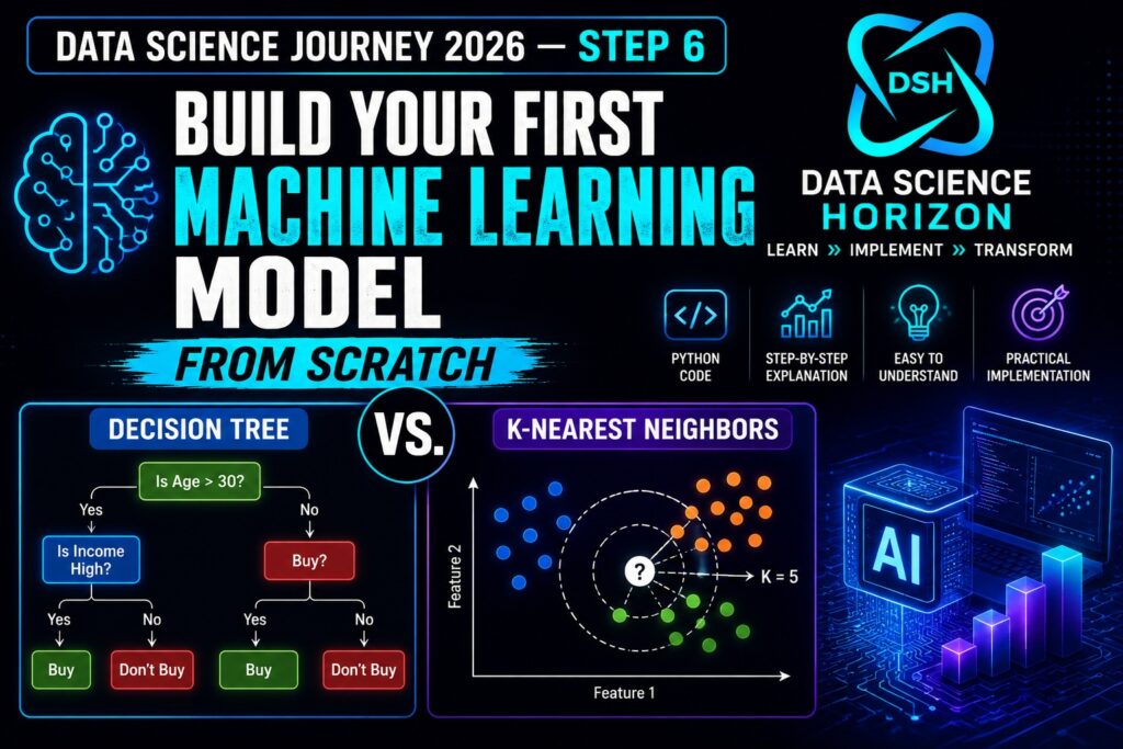
Build Your First Machine Learning Model From Scratch: Decision Tree vs. K-Nearest Neighbors
Data Science Journey 2026: Step 6
We have already learned Python, SQL, Maths: linear algebra, matrices, coordinate geometry, calculus, probability, and statistics. And we have seen the Iris dataset through Exploratory Data Analysis.
We looked at the Iris dataset from every angle: bar plots, box plots, histograms, scatter plots, a pair plot, a correlation heatmap, and concluded that “Petal Length and Petal Width” were the two features that separated the three Iris species almost perfectly.
Today, that insight finally pays off. We’re going to take it and build a step-by-step real machine learning model, train it, and evaluate it to predict on test data. We’ll train our data on two machine learning models: a Decision Tree and a K-Nearest Neighbors classifier, so you can see that the three-step scikit-learn ritual (create, fit, predict) works the same way no matter which model you reach for.
By the end of this post, you’ll have trained your first two classifiers, and you’ll understand what they’re actually doing, not just which functions to call.
What is a Machine Learning Model?
In Step 5, when we looked at the box plot of Petal Length by species, we could already tell that if Petal Length is under 2 cm, it’s almost certainly Setosa. We did that with our eyes, using graphs.
A machine learning model does the same thing, except it finds that rule automatically, from data, across four features at once instead of just one, and across millions of rows instead of just 150.
That’s the entire secret of machine learning. It isn’t magic, and it isn’t a black box. It’s pattern-finding, the same pattern-finding we were doing by hand in EDA. ML is just handed over to an algorithm so it can do it faster and at a scale you never could by hand.
A model has one job: look at inputs called features and learn a rule that predicts an output called the label or target. Today, our features are the four flower measurements: Petal Length, Petal Width, Sepal Length, and Sepal Width. Our target is the ‘Species’.
Download Jupyter Notebook
You can download the complete Jupyter Notebook from my GitHub link:
https://github.com/nidhibansal1902/Data-Science-Journey-2026
Iris Flower Dataset
We’re staying with the Iris dataset we use in EDA: 150 flowers, the 3 species: Setosa, Virginica, and Versicolor, and the 4 features you already explored. That continuity matters: you’re not learning a new dataset and a new algorithm at the same time. You already know this data inside out, so today you only need to learn what’s new, i.e., the models.
Import Libraries and load the dataset
| import pandas as pd import numpy as np import matplotlib.pyplot as plt import seaborn as sns from sklearn.model_selection import train_test_split from sklearn.tree import DecisionTreeClassifier, plot_tree from sklearn.neighbors import KNeighborsClassifier from sklearn.preprocessing import StandardScaler from sklearn.metrics import accuracy_score, confusion_matrix, classification_reportiris_df.head() |
Data Splitting: The Step Everyone Skips And Regrets
Before training anything, we need to talk about the single most important habit in machine learning: Never test a model on the same data you trained it on.
If a model studies all 150 flowers and then gets quizzed on those same 150 flowers, of course it’ll do well; it already memorized the answers. That tells you nothing about whether it can handle a new flower it’s never seen. That’s not intelligence; that’s memorization.
So we split our data into two parts: a training set (the data the model learns from) and a test set (data we hide from the model completely, used only at the end, honestly). A common split is 80% training, 20% testing, and since our dataset is perfectly balanced at 50 flowers per species, we use `stratify` to keep that balance in both sets.
| feature_cols = [‘sepal length (cm)’, ‘sepal width (cm)’, ‘petal length (cm)’, ‘petal width (cm)’] X = iris_df[feature_cols] y = iris_df[‘Species’]X_train, X_test, y_train, y_test = train_test_split( X, y, test_size=0.2, random_state=42, stratify=y)print(X_train.shape, X_test.shape) |
120 flowers to train on. 30 flowers the models will never see until judgment day. This is the foundation of every honest machine learning workflow you’ll ever build.
Algorithm 1: The Decision Tree Classifier
There are dozens of algorithms we could start with, but for a first model, we want one that thinks the way we already think, because we were doing this ourselves during EDA.
It’s called a “Decision Tree”, and here’s the entire idea in one sentence: it asks a series of yes/no questions about your features, and each answer splits the data into smaller, purer groups, until it can confidently name the species.
In EDA we looked at a box plot and said, “if Petal Length is under 2, it’s Setosa.” A Decision Tree asks exactly that kind of question, “Is Petal Length less than 2.45?” and walks down one branch if yes, another if no, asking a new question like “Is Petal Width less than 1.75?” until it lands on an answer.
Under the hood, the tree isn’t guessing which question to ask first. At every split, it tests many possible thresholds on every feature and picks the one that creates the purest possible groups, meaning each resulting group is as close to a single species as possible. There’s a name for how it measures purity: “Gini impurity”.
That’s exactly why Petal Length and Petal Width are the two features we already identified in the pair plot and the heatmap, and these are about to become the most important questions in our tree. EDA already told us where the tree would look. That’s not a coincidence; it’s the entire point of doing EDA before modeling.
Training the Decision Tree
In scikit-learn, every model follows the same three-step ritual: create it, fit it, predict with it. Once we learn this pattern, it’s identical for almost every algorithm we will ever use.
| clf = DecisionTreeClassifier(max_depth=3, random_state=42) clf.fit(X_train, y_train) |
That’s it. Three lines. “Create the model” and a tree allowed to ask at most 3 questions deep, as the max_depth value is ‘3’, so it stays simple and readable. “Fit the model”: this is where learning actually happens; the tree looks at all 120 training flowers and works out the best questions to ask.
| plt.figure(figsize=(14, 8)) plot_tree(clf, feature_names=feature_cols, class_names=clf.classes_, |
The very first question the tree chose, all on its own: “Is Petal Length less than or equal to 2.45?” That’s almost word for word the rule you found by eye in the Step 5 box plot. The model didn’t need to be told that — it discovered it, from data, in a fraction of a second.
Judging It Honestly
Now for the real test on the 30 flowers the model has never seen.
| y_pred = clf.predict(X_test) accuracy = accuracy_score(y_test, y_pred) print(f”Decision Tree Accuracy: {accuracy:.2%}”) |
On a clean, well-separated dataset like Iris, this is usually well above 90%. But accuracy alone can hide mistakes; it tells you how often you were right, not where you went wrong. For that, we need a confusion matrix.
| cm = confusion_matrix(y_test, y_pred, labels=clf.classes_) sns.heatmap(cm, annot=True, fmt=’d’, cmap=’Blues’, |
The diagonal is where the model got it right. Anything off the diagonal is a mistake and if we see any, it will almost always be a Versicolor mistaken for a Virginica, or vice versa. Why? Because we saw it during EDA, those two species overlap in Sepal measurements and, to a smaller degree, in Petal measurements too. The model’s confusion matches the exact overlap you already spotted in the scatter plot.
Which Features Actually Mattered?
Calculating which features are most important using a Decision Tree classifier.
| importances = pd.Series(clf.feature_importances_, index=feature_cols) importances.sort_values().plot(kind=’barh’, color=’#3B82F6′) plt.title(‘Which Features Did the Model Actually Use?’) plt.xlabel(‘Importance’) plt.show() |
Petal Length and Petal Width dominate. Sepal Length and Sepal Width barely matter. This is the model confirming, mathematically, the same insight your correlation heatmap and pair plot gave you in Step 5:EDA.
Algorithm 2: K-Nearest Neighbors (KNN)
A Decision Tree learns by asking questions. Our second algorithm, K-Nearest Neighbors, doesn’t ask questions at all; it learns by comparison.
Here’s the entire idea in one sentence: to classify a new flower, look at the ‘k’ flowers in the training set that are most similar to it, its “nearest neighbors” in terms of the four measurements, and let them vote. Whichever species is most common among those neighbors becomes the prediction.
Think about how you might actually do this by hand. If someone handed you a new flower’s measurements and asked “what species is this,” a completely reasonable approach is: “well, it’s really close in size to these five flowers I already know are Versicolor, so I’ll guess Versicolor too.” That’s it. That’s the whole algorithm, no tree, no splits, no impurity calculations. Just distance and a vote.
One detail matters a lot for KNN specifically: because it relies on measuring distance between flowers, features on a larger numeric scale (Sepal Length, in centimeters, versus something with more or less spread) can unfairly dominate that distance calculation. So, unlike our Decision Tree, KNN needs its features scaled first, so every feature contributes fairly.
Training the KNN Model
Same three-step ritual: create, fit, predict, just with scaling added first. Read the entire article on scaling here.
| scaler = StandardScaler() X_train_scaled = scaler.fit_transform(X_train) X_test_scaled = scaler.transform(X_test)knn = KNeighborsClassifier(n_neighbors=5) knn.fit(X_train_scaled, y_train) |
We picked n_neighbors=5, a common starting point. Each new flower will be classified by a majority vote among its 5 closest neighbors in the training set.
Judging It Honestly
Let’s predict and evaluate on the test dataset.
| y_pred_knn = knn.predict(X_test_scaled) accuracy_knn = accuracy_score(y_test, y_pred_knn) print(f”KNN Accuracy: {accuracy_knn:.2%}”)cm_knn = confusion_matrix(y_test, y_pred_knn, labels=knn.classes_) sns.heatmap(cm_knn, annot=True, fmt=’d’, cmap=’Greens’, xticklabels=knn.classes_, yticklabels=knn.classes_) plt.xlabel(‘Predicted Species’) plt.ylabel(‘Actual Species’) plt.title(‘Confusion Matrix — K-Nearest Neighbors’) plt.show() |
Try the KNN algorithm by yourself and check the results. I have shared the code here not added the results in Jupyter Notebook. Check how these two different algorithms predict and evaluate the Iris dataset.
Decision Tree vs. KNN: Which Should You Reach For?
| Decision Tree | KNN | |
| How does it decide? | Asks a sequence of yes/no questions | Votes among the most similar training examples |
| Needs feature scaling? | No | Yes |
| Easy to explain to a non-technical person? | Very Easily | Fairly |
| Training Speed | Fast | Instant |
| Prediction Speed | Very Fast | Slow on larger dataset |
| Prone to overfitting? | Yes: if left unlimited | Yes: if ‘K’ is too small |
Neither algorithm is “better” in some universal sense; they’re different tools with their individual style, with pros and cons.
The Mistake That Fools Every Beginner
One warning before we wrap up. Watch what happens if we let the Decision Tree ask unlimited questions instead of stopping at 3:
| deep_clf = DecisionTreeClassifier(max_depth=None, random_state=42) deep_clf.fit(X_train, y_train)print(“Train accuracy:”, deep_clf.score(X_train, y_train)) print(“Test accuracy:”, deep_clf.score(X_test, y_test)) |
Training accuracy often shoots up to 100%. But test accuracy doesn’t improve, and can even get worse. This is called “overfitting”. The model didn’t learn the pattern; it memorized the training flowers, including their quirks and noise. It looks perfect on data it’s already seen and shakier on anything new.
The same trap exists for KNN in the opposite direction: pick “n_neighbors=1,” and the model will happily “memorize” every training point as its own nearest neighbor, hitting near-100% training accuracy while becoming overly sensitive to noise on new data. This is exactly why we hid the test set in the first place; otherwise, you will walk away thinking you’d built a perfect model, when really you’d just built a very good memory.
Stay Tuned!!
Congratulations! You have just built your first Machine Learning Model.
Explore the complete Data Science Series with article links, Jupyter notebooks, and YouTube links mentioned below:
Keep learning and keep implementing!!

