t-distributed Stochastic Neighbor Embeddings (t-SNE)

Table of Contents

1. What is the t-SNE Algorithm?
2. Aim of  t-SNE
3. Usage
4. Science behind t-SNE
5. Python Code with Results
6. Limitation
7. Conclusions

What is t-SNE Algorithm?

The term “t-Distributed Stochastic Neighbor Embeddings” (t-SNE) refers to a non-linear, unsupervised method of reducing the dimensionality of high-dimensional data through exploration and visualization.

t- distributed Stochastic: The similarity between two points in a low-dimensional space is computed using the Student’s T-distribution with one degree of freedom.

Neighbor: Similarity is preserved based on neighborhood distance.

Embedding: For every point in d-dimensional data, we can create a point in 2-D.

Aim of t-SNE

The main aims of the t-SNE algorithm are:

• Dimensionality Reduction

We have data with so many features that somewhere exists in d-dimensional space. It’s very difficult to understand and explore that data. So, with the dimensionality reduction technique, data is reduced to 2-D or 3-D, so that information in data is at minimal loss.

• Data Visualization

As data is reduced to 2-D using t-SNE, data can be easily visualized using scatter plots, mainly. When data is non-linear and cannot be separated using a straight line, then t-SNE helps in separating the data and visualizing it beautifully.

• Clustering

t-SNE is implemented on unsupervised data and used for clustering purposes.

• Anomalies Detection

To detect anomalies and outliers in the data.

Usage

t-SNE is mainly used for complicated datasets and has a wide range of applications, like:

• Image Processing
• Natural Language Processing (NLP)
• Speech Recognition
• Music Analysis
• Biomedical Signal Processing
• Cancer Research
• Geological Domain Interpretation

Science behind t-SNE

In both higher and lower dimensional space, the t-SNE algorithm determines the similarity measure between pairs of instances. It then attempts to optimize two similarity metrics.  It does all of that in three steps. 

1. t-SNE models a point being selected as a neighbor of another point by calculating a pairwise similarity between all data points in the high-dimensional space using a Gaussian kernel. The points that are near are assigned a higher probability, and the points that are far apart have a lower probability.
2. Then, the t-SNE algorithm tries to define a similar probability distribution in a low-dimensional map and map higher dimensional data points onto lower dimensional space while preserving the pairwise similarities. 
3. It is achieved by minimizing the Kullback–Leibler divergence (KL divergence) between the probability distribution of the original high-dimensional and lower-dimensional. The algorithm uses gradient descent to minimize the divergence. The algorithm is trying to reach an optimal stable state for the lower-dimensional embedding.

To perceive and comprehend the structure and relationships in the higher-dimensional data, the optimization process enables the formation of clusters and sub-clusters of related data points in the lower-dimensional space.

Python Code with Results

After learning the fundamentals and the science of the t-SNE technique, let’s examine a Python code example that uses t-SNE to analyze an actual MNIST dataset.

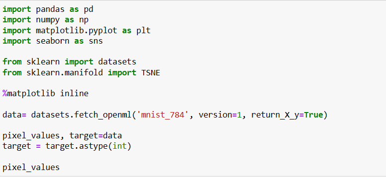
We will be using sci-kit-learn’s sklearn.manifold.TSNE module to implement TSNE on the MNIST dataset.

Step 1:

Import the required libraries and load the MNIST dataset. We will get data in ‘pixel_values’ with 70000 rows and 784 columns. Column values are pixel values of images with a dimension of 28*28. ‘target’ is the integer type target variable.

Output>>

Step 2:

Let’s plot an image of a sample using Matplotlib.

Step 3:

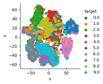
Implement t-SNE with n_components=’2’ (data will be converted to 2 dimensional), perplexity=’50’, and n_iters=’5000’ on a sample of 5000 data points. Create a new data frame ‘tsne_df’ with new dimensions and target to plot a scatter plot.

Step 4:

A 2-D scatter plot is plotted with ‘Dim_1’ at the x-axis and ‘Dim_2’ at the y-axis and the target value as a color legend.

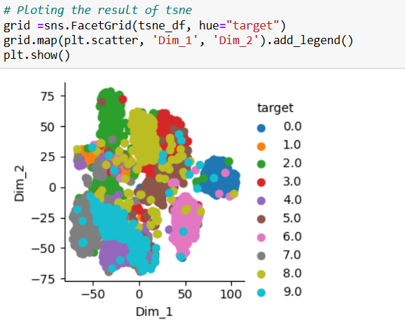
We can see a beautiful scatter plot with 10 different target values.

Hyperparameters

Two hyperparameters in t_SNE can be tuned for better performance.

1. Iterations (n_iter): The maximum number of iterations for the optimization. The default value is 1000.
2. Perplexity: The perplexity is related to the number of nearest neighbors that are used in other manifold learning algorithms. Larger datasets usually require greater perplexity.

Note: Never run t-SNE once. Try with different combinations of hyperparameters.

Limitation

The crowding problem is an issue that sometimes arises in t-SNE. Preserving the distance in every neighborhood (N) isn’t always feasible. We refer to this kind of issue as a crowding problem.

Conclusions

t-distributed Stochastic Neighbor Embedding is a non-linear dimensionality reduction and visualization technique that can be easily implemented in Python using the scikit-learn library. We can learn machine learning concepts easily with hands-on Python code. Give it a try and run the code by yourself.

Stay Tuned

Do you want to become a data scientist? Click here for detailed information.

Keep learning and keep implementing!!