
In this article, we will predict introverts from extroverts using Machine Learning Algorithms to gain a deeper understanding of human behavior and personality.
1. Introduction
This is a playground dataset that I have used to predict introverts from extroverts, analyzing different personality traits. Using Machine Learning algorithms helps in understanding various personality traits of introverts and extroverts, like:
- Extroverts like to socialize more and interact with people more.
- Introverts think before speaking, and extroverts think after speaking.
- Introverts prefer small, closed groups while extroverts are often seen in large groups.
- Extroverts post more regularly on social platforms.
Overall, predicting introverts from extroverts is important to learn more about human behaviour.
2. Data Source
The data source for “Predicting Introverts from Extroverts” is taken from Kaggle. Click here for the dataset.
In the data source, we have three CSV files:
train.csv – the training dataset; ‘Personality’ is the target variable.
test.csv – the test dataset; your objective is to predict the ‘Personality’ variable.
sample_submission.csv – a sample submission file in the correct format
3. Objective
The objective is to predict whether a person is an Introvert or an Extrovert, given their social behavior and personality traits. Evaluation will be done on the Accuracy Score. The goal is to predict the target variable ‘Personality’ for test data and submit it in ‘sample_submission.csv’ format.
4. Evaluation Metrics
Submissions are evaluated on Accuracy between the predicted value and the observed target.
5. Data Understanding
Let’s understand the dataset in detail with Python Code.
Import Libraries
The first step is to import relevant libraries.
Code to import libraries
| import pandas as pd import numpy as np import matplotlib.pyplot as plt import seaborn as sns import plotly.express as px import category_encoders as ce from sklearn.model_selection import train_test_split from sklearn.metrics import confusion_matrix from sklearn import metrics from sklearn.metrics import roc_curve, auc from sklearn.tree import DecisionTreeClassifier from sklearn.ensemble import RandomForestClassifier from sklearn.model_selection import GridSearchCV from sklearn.preprocessing import StandardScaler from catboost import CatBoostClassifier from xgboost import XGBClassifier from sklearn.model_selection import train_test_split from sklearn.metrics import accuracy_score from sklearn.metrics import classification_report |
Loading Data
Load train, test, and sample_submission CSV files.
Code to load data
| df_train= pd.read_csv(“/kaggle/input/playground-series-s5e7/train.csv”) df_test = pd.read_csv(“/kaggle/input/playground-series-s5e7/test.csv”) df_sub = pd.read_csv(“/kaggle/input/playground-series-s5e7/sample_submission.csv”) print(“Shape of training data: “,df_train.shape) print(“Shape of test data: “,df_test.shape) print(“Shape of submission file: “,df_sub.shape) print(“Print columns data “, df_train.columns.values) |
Output
| Shape of training data: (18524, 9) Shape of test data: (6175, 8) Shape of submission file: (6175, 2) Print columns data [‘id’ ‘Time_spent_Alone’ ‘Stage_fear’ ‘Social_event_attendance’ ‘Going_outside’ ‘Drained_after_socializing’ ‘Friends_circle_size’ ‘Post_frequency’ ‘Personality’] |
Data Description
Training data has 18524 rows of data with 9 columns, out of which 8 are independent features and ‘Personality’ is a dependent feature or target variable described below:
id: Denotes serial no.
Time_spent_Alone: No. of hours spent alone.
Stage_fear: fear of the stage: Yes or No
Social_event_attendance: Attendance in any social event.
Going_outside: Frequency of going out.
Drained_after_socializing: Is the person drained after socializing: Yes or No
Friend_circle_size: Size of the friend circle.
Post_frequency: Frequency of social media posts.
Personality: It is the target variable that denotes the personality of a person: Introvert or Extrovert
Data Cleaning
Understand data types for all features and check for missing and duplicate values.
Code to get train data info
| df_train.info() |
Output
| <class ‘pandas.core.frame.DataFrame’> RangeIndex: 18524 entries, 0 to 18523 Data columns (total 9 columns): # Column Non-Null Count Dtype — —— ————– —– 0 id 18524 non-null int64 1 Time_spent_Alone 17334 non-null float64 2 Stage_fear 16631 non-null object 3 Social_event_attendance 17344 non-null float64 4 Going_outside 17058 non-null float64 5 Drained_after_socializing 17375 non-null object 6 Friends_circle_size 17470 non-null float64 7 Post_frequency 17260 non-null float64 8 Personality 18524 non-null object dtypes: float64(5), int64(1), object(3) memory usage: 1.3+ MB |
Code to check for duplicate values
| df_train.duplicated().sum() |
Output
| 0 |
Observations
- Output Feature: Personality (Categorical): two values possible: ‘Extrovert’ and ‘Introvert’
- Numerical Features: ‘Time_spent_Alone’, ‘Social_event_attendance’, ‘Going_outside’, ‘Friends_circle_size and ‘Post_frequency’. These are discrete numerical features.
- Categorical Features: ‘Stage_fear’ and ‘Drained_after_socializing’ both are nominal, so label encoding can be used.
- There seems to be no outliers in numerical features Time_spent_Alone, Social_event_attendance, Going_outside, Friends_circle_size and Post_frequency
- There are many Nan values in features: ‘Time_spent_Alone’,’Stage_fear’, ‘Social_event_attendance’, ‘Going_outside’, ‘Drained_after_socializing’, ‘Friends_circle_size’and ‘Post_frequency’
- There are no duplicate values.
Code to handle null values in ‘Time_spent_Alone’
| median_Time_spent_Alone = df_train.groupby(“Personality”)[“Time_spent_Alone”].median() print(median_Time_spent_Alone ) df_train[‘Time_spent_Alone’] = df_train.apply( lambda row: median_Time_spent_Alone[row[‘Personality’]] if pd.isnull(row[‘Time_spent_Alone’]) else row[‘Time_spent_Alone’], axis=1) |
Output
| Personality Extrovert 2.0 Introvert 7.0 Name: Time_spent_Alone, dtype: float64 |
Observations
- Median values for extrovert personality are 2.0, which he spent alone.
- Median values for introvert personality are 7.0, which he spent alone.
You can handle other null values for numerical features like this and categorical features with the mode value. To see the full code, kindly go to the Kaggle notebook.
6. Exploratory Data Analysis and Visualizations
Now is the time for data exploratory analysis and visualizations. Let’s start with Univariate analysis to find statistical features like the mean, median, standard deviation, percentile, quantile, and skewness of numerical features.
Code for Univariate Analysis
| df_train.describe() #It will do univariate analysis on numerical features only |
Output
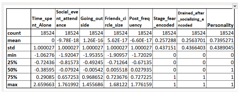 |
Observations
- Numerical Features: ‘Time_spent_Alone’, ‘Social_event_attendance’, ‘Going_outside’, ‘Friends_circle_size and ‘Post_frequency’. These are discrete numerical features.
- Categorical Features: ‘Stage_fear’ and ‘Drained_after_socializing’ both are nominal, so label encoding can be used.
- There seems to be no outliers in numerical features Time_spent_Alone, Social_event_attendance, Going_outside, Friends_circle_size, and Post_frequency
- Data is highly skewed towards ‘Extroverts’.
Code to find unique categorical values
| def find_unique(feature): print(“Unique features of “+ feature + “: “,df_train[feature].unique()) for column in df_train[[‘Time_spent_Alone’, ‘Stage_fear’, ‘Social_event_attendance’, ‘Going_outside’ ,‘Drained_after_socializing’ ,‘Friends_circle_size’, ‘Post_frequency’, ‘Personality’]]: find_unique(column) |
Output
| Unique features of Time_spent_Alone: [ 0. 1. 6. 3. 2. 4. 5. 9. 10. 7. 8. 11.] Unique features of Stage_fear: [‘No’ ‘Yes’] Unique features of Social_event_attendance: [ 6. 7. 1. 4. 8. 2. 5. 0. 9. 3. 10.] Unique features of Going_outside: [ 4. 3. 0. 5. 1. 6. 2. 7.] Unique features of Drained_after_socializing: [‘No’ ‘Yes’] Unique features of Friends_circle_size: [15. 10. 3. 11. 13. 4. 0. 14. 5. 9. 12. 8. 2. 1. 6. 7.] Unique features of Post_frequency: [ 5. 8. 0. 3. 4. 2. 9. 10. 6. 7. 1.] Unique features of Personality: [‘Extrovert’ ‘Introvert’] |
Observations
- Numerical features are discrete.
- Categorical Features are binary.
- ‘Time_spent_Alone‘ has 12 unique numerical values.
- ‘Social_event_attendance‘ has 11 unique numerical values.
- ‘Going_outside’ has 8 unique numerical values.
- ‘Friends_circle_size’ has 16 unique numerical values.
- ‘Post_frequency’ has 11 unique numerical values.
- ‘Stage_fear’ has two values: Yes and No.
- ‘Drained_after_socializing’ has two values: Yes and No.
- ‘Personality’ has two values: Extrovert and Introvert.
Let’s draw a histogram to understand the division of the target variable ‘Personality’.
Code to draw ‘Personality’ histogram
| fig = px.histogram(df_train, x=‘Personality’,barmode=‘group’,title=“Personality Histogram”) fig.show() |
Output
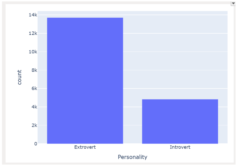 |
Observation
- Data is highly skewed towards the ‘Extrovert’ personality.
Code to draw a Bar Chart of ‘time_spent_alone’ as per ‘Personality’
| fig = px.histogram(df_train, x=‘Time_spent_Alone’,color=“Personality”,barmode=‘group’,title=“Grouped Bar Chart of Time_spent_Alone”) fig.show() |
Output
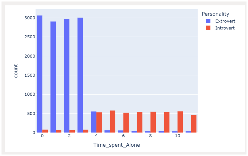 |
Observations
- Persons with an ‘Extrovert’ personality spend less than 4 hours alone.
- Persons with an ‘Introvert’ personality spent 4-11hours alone.
7. Feature Engineering
Now is the time for Feature Engineering for various features and aligning them so that our machine learning model performs well.
Label Encoding
We will first label encode the categorical features Stage_fear, Drained_after_socializing, and Personality.
Code to label encode in ‘Stage_fear, ‘Drained_after_socializing and Personality.
| # Label encode: yes → 1, no → 0 df_train[‘Stage_fear_encoded’] = df_train[‘Stage_fear’].map({‘Yes’: 1, ‘No’: 0}) df_train[‘Drained_after_socializing_encoded’] = df_train[‘Drained_after_socializing’].map({‘Yes’: 1, ‘No’: 0}) df_train[‘Personality_encoded’] = df_train[‘Personality’].map({‘Extrovert’: 1, ‘Introvert’: 0}) |
Output
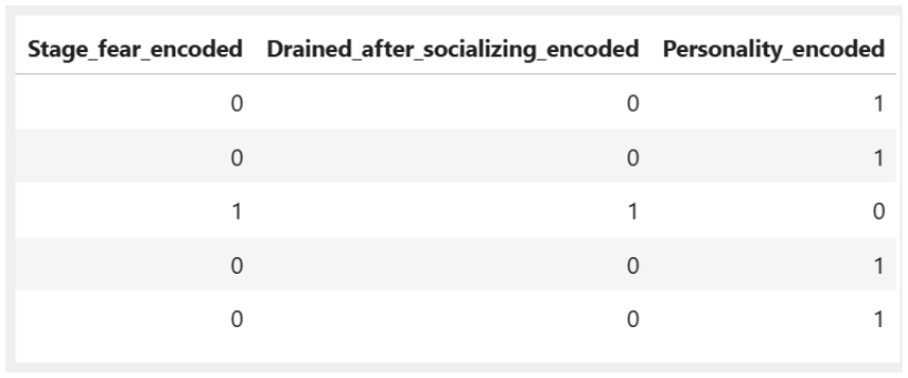 |
Observation
- Categorical value ‘Yes’ encoded to ‘1’ and ‘No’ to ‘0’
- Categorical value ‘Extrovert’ encoded to ‘1’ and ‘Introvert’ to ‘0’
Feature Standardization
We will standardize all numerical features using Standard Scaler.
Code to standardize all numerical features.
| # Standardize all numerical features numerical_features = [‘Time_spent_Alone’,‘Social_event_attendance’, ‘Going_outside’, ‘Friends_circle_size’, ‘Post_frequency’] scaler = StandardScaler() df_train[numerical_features] = scaler.fit_transform(df_train[numerical_features]) df_train.head() |
Output
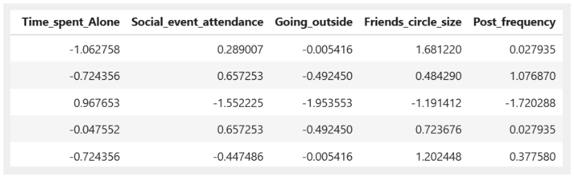 |
Observation
- All numerical features are standardized with a ‘0’ mean and a standard deviation of ‘1’.
Handle Test Data
- Handle null values and duplicate values in test data (df_test.csv).
- Do all feature engineering steps on test data.
8. Machine Learning Algorithms Implementation
Once all data is cleaned, processed, and feature engineered, now is the time for machine learning algorithm implementation.
Data Splitting
Let’s split ‘df_train’ into 70% training data and 30% validation data to train for machine learning algorithm.
Code to split data into training data and validation data.
| y=df_train[‘Personality_encoded’] X= df_train.drop(‘Personality_encoded’,axis=1) X_train, X_val, y_train, y_val = train_test_split(X, y, test_size=0.3, random_state=42) |
Machine Learning Algorithm Implementation
We have implemented XGBoostClassifier with tuned parameters.
Code to model training data using XGBoostClassifier
| model_xg = XGBClassifier(max_depth = 10, n_estimators = 100, learning_rate=0.01, colsample_bytree= 0.7, subsample= 0.7,reg_alpha =0.01, random_state=42, n_jobs=-1) model_xg.fit(X_train, y_train) # Predict y_pred_xg = model_xg.predict(X_val) # Evaluate report_xg = classification_report(y_val, y_pred_xg) print(report_xg) |
Output
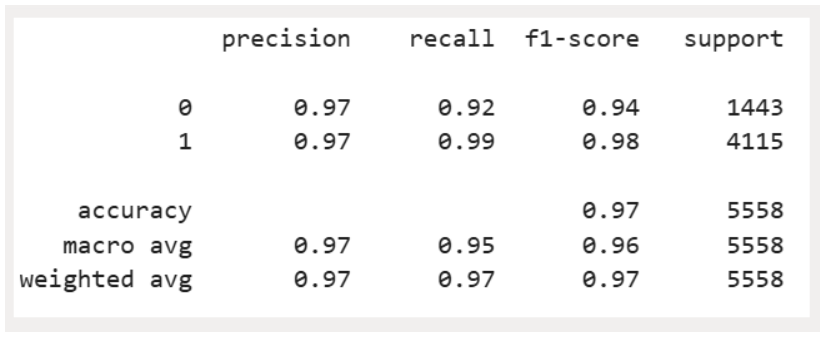 |
Observation
- We get a detailed classification report, and XGBoost performs very fast.
- XGBoost performs very well with an accuracy of 97% achieved on validation data.
Finding important features
Let’s find out the most and least important features in the dataset learned by XGBoostClassifier
Code to find important features using an XGBoostClassifier trained model
| xgb.plot_importance(model_xg, max_num_features=10) plt.show() |
Output
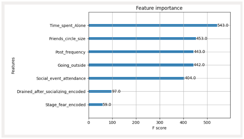 |
Observations
- ‘Time_spent_Alone’ is the most important feature.
- ‘Drained_after_socializing’ and ‘Stage_fear’ are the least important features.
9. Results
Now, predict the output on test data (df_test) and submit the results in the ‘submission.csv’ file.
Accuracy achieved on unknown test data is ‘0.973279’ on Kaggle.
Kaggle Notebook Link:
Click on the link below for the complete notebook, and kindly upvote if you like and learn from this notebook. Also, drop a comment and any queries you have.
https://www.kaggle.com/code/playingmyway/simplified-predict-introverts-from-extroverts
Stay Tuned!!
Learn the complete data science project lifecycle by clicking on the link below:
Keep learning and keep implementing!!


Pingback: Multi-Class Prediction of Obesity Risk- Kaggle Dataset - Data Science Horizon
Very good article
Thanks dear