Introduction
In this article, we are covering 3 scenarios of skewed data and implementing feature engineering for them:
- When data is highly right-skewed
- When data is highly left-skewed
- When data spikes at extreme values
Dataset Information
Data is taken from the Kaggle Dataset “Predicting the Beats-per-Minute of Songs”. Click on the link below for the dataset:
https://www.kaggle.com/competitions/playground-series-s5e9/data
Handling Different Scenarios
Let’s discuss how to handle these 3 different scenarios in detail:
1. Right-Skewed Feature Data
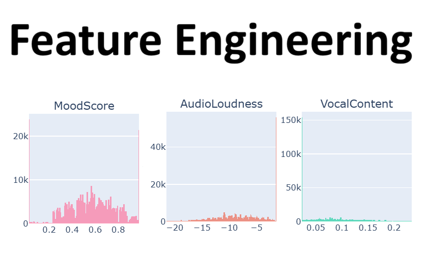
The feature ‘Vocal Content’ is highly right-skewed, with a significant spike at the minimum value and a long tail.

Here, approximately 30% of data values are equal to the minimum value, and the rest is distributed from 0.03 to 0.25. To handle such right-skewed data, a new binary feature is created that flags whether a value belongs to the min-value spike group or not by implementing the code below:
# Extract minimum threshold value
threshold = df['VocalContent'].min()

# Create a binary indicator
df["VocalContent_bin"] = df['VocalContent'].apply(lambda x: 0 if (x <= threshold) else 1).astype(int)
Distribution of ‘Vocal Content’ after converting into a binary feature:

2. Left-Skewed Feature Data
The feature ‘Audio Loudness’ is highly left-skewed, with a significant spike at the maximum value and a long tail on the left side.

Here, approximately 11% of data values are equal to the maximum value, and the rest is distributed. To handle such left-skewed data, a new binary feature is created that flags whether a value belongs to the max-value spike group or not by implementing the code below:
# Extract minimum threshold value
threshold = df['AudioLoudness'].max()

# Create a binary indicator
df["AudioLoudness_bin"] = df['AudioLoudness'].apply(lambda x: 1 if (x >= threshold) else 0).astype(int)
Distribution of ‘Audio Loudness’ after converting into a binary feature:

3. Data spikes at extreme values
The ‘MoodScore’ feature exhibits a significant spike at both the minimum and maximum values, along with a long tail in between.

Here, approximately 9% of data values are equal to the minimum and maximum values, and the rest is distributed between them. To handle this type of skew, we have added a binary feature indicator to mark whether a row belongs to the extreme group, either a very low or a very high mood score, by implementing the code below:
# Define thresholds for "low" or "high" spikes
low_threshold = df['MoodScore'].min() # near 0
high_threshold = df['MoodScore'].max() # near 1

# Create binary indicators
df["MoodScore_is_low"] = (df["MoodScore"] <= low_threshold).astype(int)
df["MoodScore_is_high"] = (df["MoodScore"] >= high_threshold).astype(int)

# Create a combined indicator for "extreme"
df["MoodScore_extreme"] = ((df["MoodScore"] <= low_threshold) | (df["MoodScore"] >= high_threshold)).astype(int)
Distribution of ‘Mood Score’ after converting into a binary feature:

Conclusion
We need to be experimental in handling different kinds of features. Defined formulas won’t work for every feature. And, trust me, various types of feature engineering have a significant impact even on a simple model.
Stay Tuned!!
Learn to do the multi-class prediction of obesity risk on a Kaggle dataset in detail by clicking on the link below:
Keep learning and keep implementing!!

