
Statistics for Data Science
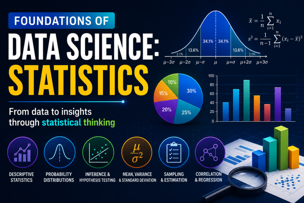
Every data scientist works with Statistics every single day. It is the tool that transforms raw numbers into confident decisions.
Where Probability tells you how likely something is to happen, Statistics tells you what the data you have already collected actually means and whether the patterns you see in it are real or just noise.
What is Statistics?
Statistics is the mathematical science of collecting, organising, analysing, interpreting, and presenting data. Statistics is broadly divided into two main branches:
1. Descriptive Statistics
Descriptive Statistics summarises and describes the characteristics of a dataset. It answers the question: “What does my data look like?”
Real-world Example: Calculating the average salary of data scientists in India, the most common job title across companies, and how spread out those salaries are – that is descriptive statistics.
2. Inferential Statistics
Inferential Statistics concludes a larger population based on a smaller sample. It answers the question: “What can I conclude from what I have seen?”
Real-world Example: You survey 1,000 students about their preferred programming language and use Statistics to conclude what 10 million students likely prefer – that is inferential statistics.
“Descriptive Statistics describes what you have. Inferential Statistics predicts what you do not yet know.”
Why Statistics Matters in AI?
There are 3 core reasons for statistics to be played important role in AI and Machine Learning:
1. Data Understanding
Before building any model, you must understand the distribution, spread, and shape of your data. All of this comes from descriptive statistics applied during Exploratory Data Analysis.
2. Decision Making
The p-value, confidence interval, and correlation coefficient are statistical tools used in every real-world ML project. They translate raw numbers into confident decisions.
3. Model Validation
Statistics tells you whether your model’s performance is genuinely better or just a lucky result on one particular test set.
Core Statistics Concepts Every Data Scientist Must Know
There are 6 core statistical concepts that every data scientist must know:
1. Measures of Central Tendency
Central tendency describes the centre of a dataset around which most data points cluster.
“Mean” is the arithmetic average, i.e., the sum of all values divided by the total count.
Mean (μ) = (x₁ + x₂ + x₃ + … + xₙ) / n
“Median” is the middle value when data is sorted in order. It is more robust than the mean when outliers are present.
“Mode” is the most frequently occurring value in the dataset. A dataset can be unimodal (one mode), bimodal (two modes), or multimodal.
Real-world Example: If five data scientists earn ₹8L, ₹9L, ₹10L, ₹11L, and ₹50L per year:
– Mean = ₹17.6L, pulled upward by the ₹50L outlier.
– Median = ₹10L, a far more honest picture of what a typical data scientist earns.
Always check for outliers before choosing between mean and median. Outliers pull the mean away from the true centre but the median stays honest.
2. Measures of Spread
Measures of spread describe how much variation exists in your data and how far values are from the centre.
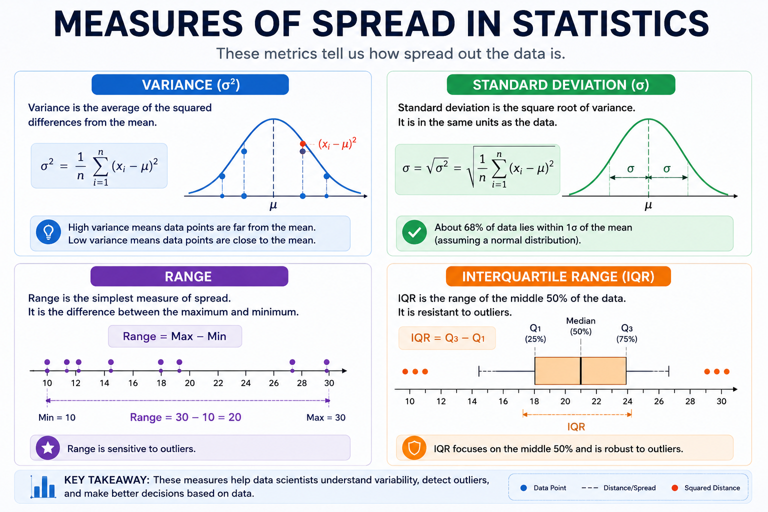
Variance measures the average squared deviation of each data point from the mean.
Variance (σ²) = Σ(xᵢ – μ)² / n
Standard Deviation is the square root of variance; it returns the measure to the original unit of the data, making it interpretable.
Standard Deviation (σ) = √Variance
Range is simply the maximum value minus the minimum value, a quick but outlier-sensitive measure of spread.
Interquartile Range (IQR) is the range of the middle 50% of your data, from the 25th percentile (Q1) to the 75th percentile (Q3). IQR is the standard method for detecting outliers.
IQR = Q3 – Q1
Outlier if: Q1 – 1.5 × IQR > value > Q3 + 1.5 × IQR
A small standard deviation means data clusters tightly around the mean. A large one means data is widely spread and your ML model will carry higher uncertainty in its predictions.
3. Hypothesis Testing
Hypothesis Testing is the most important statistical tool in a data scientist’s toolkit. It determines whether a pattern observed in data is real or could have occurred purely by random chance. It is a 4-step process:
Step 1: State the hypotheses
Null Hypothesis (H₀): There is no effect or no difference. This is what we assume to be true until the evidence proves otherwise.
Alternative Hypothesis (H₁): There is an effect or a difference. This is what we are trying to prove.
Step 2: Choose a significance level (α)
It is a threshold probability used to decide whether to reject H₀ or not. The most common value is α = 0.05; we accept a 5% chance of wrongly rejecting H₀.
Step 3: Calculate the p-value
The p-value is the probability of observing results as extreme as ours, assuming H₀ is true. If p ≤ α, the result is statistically significant
Step 4: Make a decision
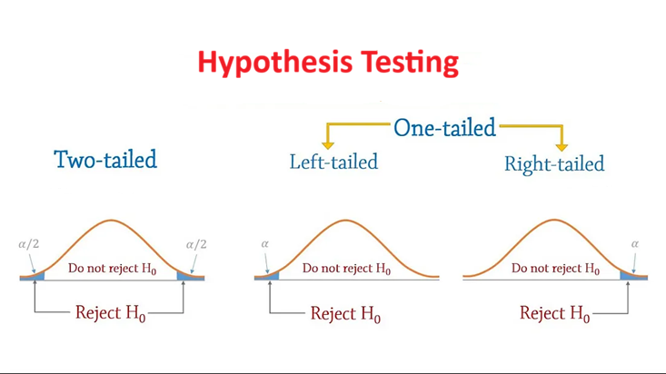
From the above image, we can say that:
p-value < α (0.05) or p-value > α (0.05) → Reject H₀ → Result is statistically significant
Else, do not reject H₀ → Result is NOT statistically significant
Real-world Example: You train a new ML model. It scores 87% accuracy versus the old model’s 85%. Is that 2% improvement real or just luck on this particular test set? Hypothesis testing answers that question.
Common hypothesis tests used in data science:
| Test | When to Use |
| One-sample t-test | Compare sample mean to a known value |
| Two-sample t-test | Compare means of two independent groups |
| Paired t-test | Compare means of the same group before and after |
| ANOVA | Compare means of three or more groups simultaneously |
| Chi-square test | Test relationship between categorical variables |
| Z-test | Large samples: comparing proportions |
A low p-value does not always mean your result is important; it means it is unlikely to have occurred by chance. Always combine statistical significance with practical significance.
4. Confidence Intervals
A Confidence Interval (CI) gives a range of values within which the true population parameter is likely to fall, at a specified level of confidence.
CI = x̄ ± Z × (σ / √n)
Where:
– x̄ = sample mean
– Z = Z-score for chosen confidence level (1.96 for 95% CI)
– σ = standard deviation
– n = sample size
Real-world Example: A model achieves 87% accuracy on the test set. A 95% confidence interval of [84%, 90%] means we are 95% confident the true accuracy on completely unseen data falls between 84% and 90%.
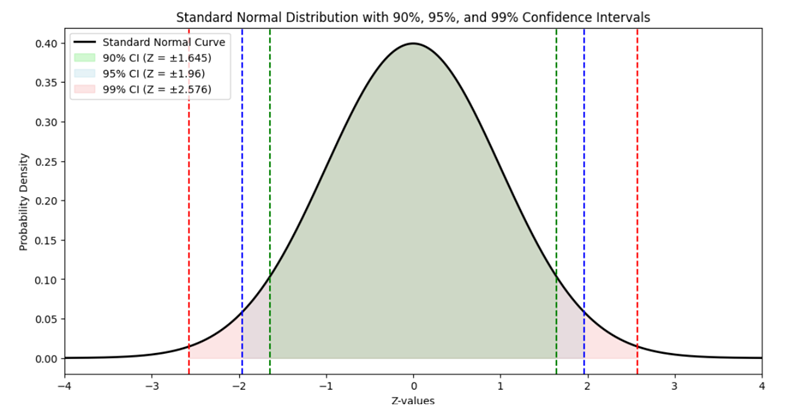
| Confidence Level | Z-score | Explanation |
| 90% | 1.645 | 90% confident that the true parameter will fall in a ±1.645 interval of the z-score. |
| 95% | 1.960 | 95% confident that the true parameter will fall in a ±1.960 interval of the z-score. |
| 99% | 2.576 | 99% confident that the true parameter will fall in a ±2.576 interval of the z-score |
A wider confidence interval means more uncertainty. Increasing sample size narrows the interval more data always means more certainty.
5. Correlation
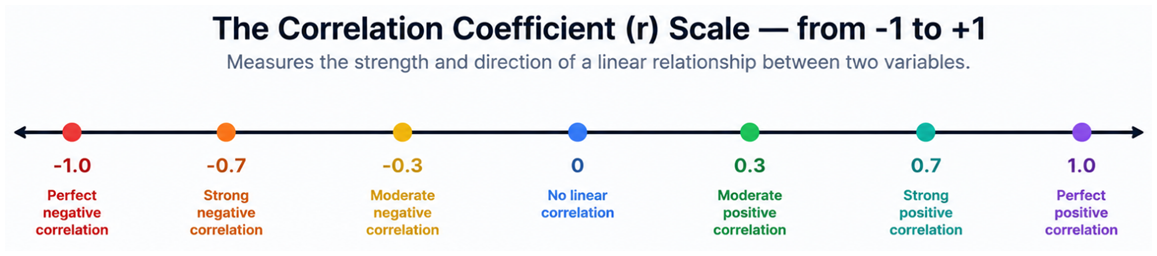
Correlation measures the strength and direction of the linear relationship between two variables.
Pearson Correlation Coefficient (r):
Pearson’s correlation coefficient is used to define the relationship between two variables; it is the covariance of the two variables divided by the product of their standard deviations.
r = Σ[(xᵢ – x̄)(yᵢ – ȳ)] / √[Σ(xᵢ – x̄)² × Σ(yᵢ – ȳ)²]
The value of r ranges from −1 to +1:
Spearman Rank Correlation Coefficient
It is used when data is not normally distributed or when working with ordinal variables. It measures correlation between the ranks of values rather than the values themselves.
![{\displaystyle r_{s}=\operatorname {\rho } {\bigl [}\ \operatorname {R} [X],\operatorname {R} [Y]\ {\bigr ]}={\frac {\ \operatorname {cov} {\bigl [}\ \operatorname {R} [X],\operatorname {R} [Y]\ {\bigr ]}\ }{\ \sigma _{\operatorname {R} [X]}\ \sigma _{\operatorname {R} [Y]}\ }},}](https://wikimedia.org/api/rest_v1/media/math/render/svg/260a8b5244863c3953fbe12b18022f8fe917c5c2)
where denotes the conventional Pearson correlation coefficient operator, but applied to the rank variables.

Correlation does not imply causation. Ice cream sales and drowning incidents are strongly correlated because both increase in summer. But, the ice cream sales did not cause the drowning. Always think carefully about why two variables are related before concluding one causes the other.
6. Linear Regression: The Bridge to Machine Learning
Linear Regression models the relationship between a dependent variable (y) and one or more independent variables (x). It is the direct bridge between Statistics and Machine Learning.
Simple Linear Regression
y = mx + c
Where:
– y = dependent variable: what we are predicting
– x = independent variable: the input feature
– m = slope: how much y changes for each unit change in x
– c = intercept: value of y when x = 0
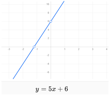
This is a straight line with:
Slope (m) = 5
Y-intercept (c) = 6
How the model finds m and c: It minimises the Sum of Squared Residuals (SSR) — the total squared difference between actual and predicted values. This minimisation uses derivatives from Calculus to find the optimal m and c. This is the exact point where Statistics and Calculus meet.
R² (R-squared)
It measures how well the regression line fits the data; it means how close the predicted value is to the actual values:
R² = 1 – (SSR / SST)
- SSR: The Sum of Residual Squares (the unexplained variance or distance between actual data and the regression line).
- SST: The Total Sum of Squares (the total variance or distance between actual data and the overall average)
– R² = 1.0 → perfect fit and model explains all variance
– R² = 0.85 → model explains 85% of the variance in y
– R² = 0.0 → model explains nothing
R² tells you how much of the outcome your features explain. A high R² on training data and low R² on test data is a sign of overfitting, a statistical red flag every data scientist must watch for.
Statistics in Python: Hands-On
You do not need to solve statistical formulas by hand as a data scientist. Python libraries handle the computation. I have uploaded a complete Jupyter Notebook on GitHub; click on the link below:
Stay Tuned!!
Congratulations! You now understand all the important mathematical foundations of Data Science.
Statistics is one of the mathematical foundations every data scientist needs. Explore the complete series:
- Linear Algebra
- Coordinate Geometry
- Planes
- Matrices
- Calculus
- Probability
- Statistics – you are here
Keep learning and keep implementing!!

