
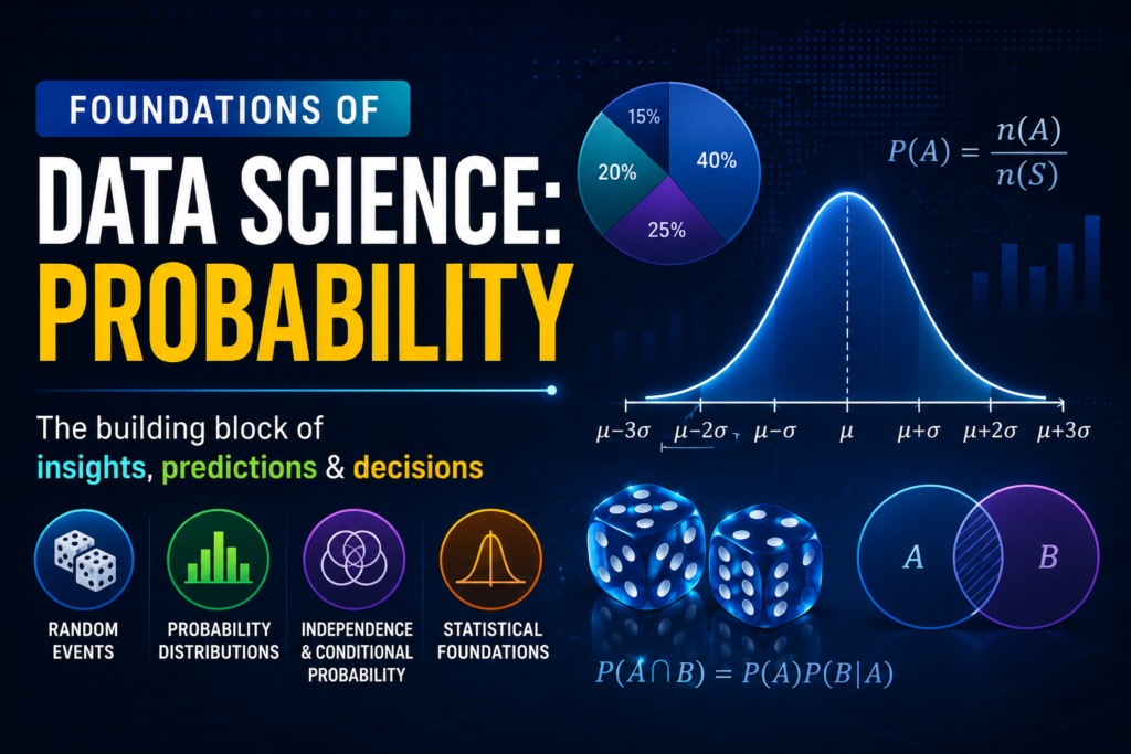
Probability for Data Science
Probability is the mathematical study of uncertainty and likelihood. Linear Algebra deals with static data structures, Calculus measures how fast things change, and Probability answers the most fundamental question in all of data science: “How confident are we?”
Probability for Data Science is one of the most important mathematical foundations every aspiring data scientist should master. Every Machine Learning model does not predict facts; it predicts probabilities. A spam filter does not say “this is spam.” It says “there is a 94% chance this is spam.” Understanding probability is not optional for a data scientist; it is the language your models speak.
A. What is Probability in Data Science?
Probability is a number between 0 and 1 that measures the likelihood of an event occurring.
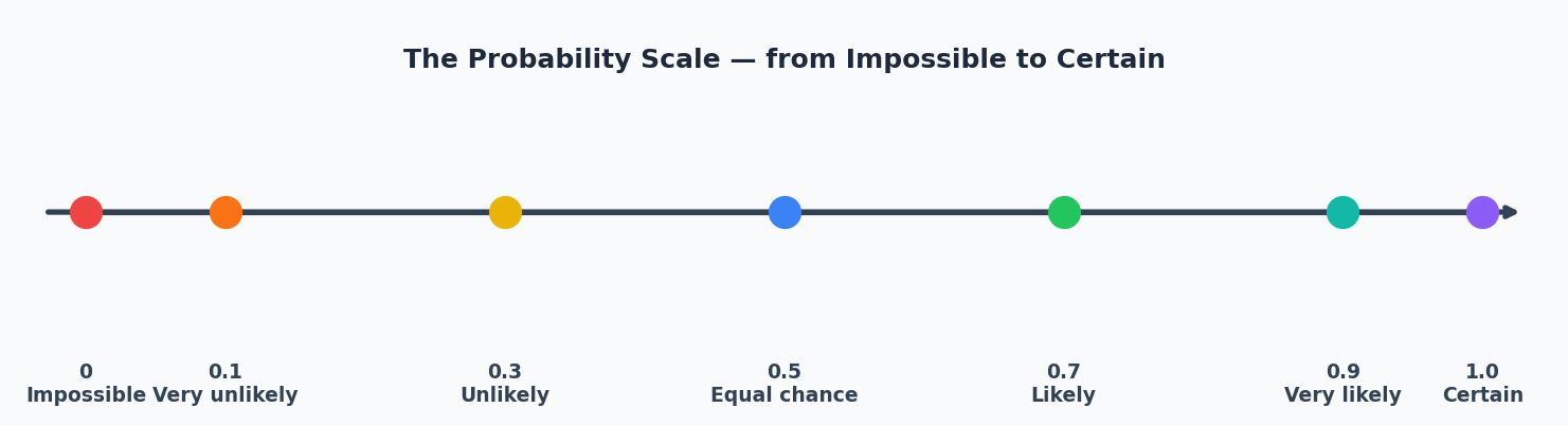
The image shows the probability scale: 0 = impossible, 1 = certain, and in data science, everything lives in between.
1. Theoretical Probability
Theoretical probability is calculated using mathematical reasoning, without running experiments. It is based on what we expect to happen in a perfectly ideal situation.
Real-world Example: Rolling a fair die, the theoretical probability of getting a 6 is 1/6 = 0.167, because there is one favourable outcome out of six equally likely outcomes.
2. Experimental Probability
Experimental probability is calculated from actual observed data by running real experiments and recording outcomes.
Real-world Example: You roll a die 1,000 times and get a 6 exactly 178 times. The experimental probability is 178/1000 = 0.178.
As the number of experiments increases, experimental probability converges toward theoretical probability. This is the Law of Large Numbers: one of the most important ideas in Machine Learning.
B.Why Does Probability Matter in Machine Learning and AI?
Probability matters in AI and Machine Learning for 3 core reasons:
1. Uncertainty Quantification
Real-world data is never perfect. Probability gives your model a principled way to express uncertainty rather than forcing it to give one definitive answer.
2. Model Training
Many ML algorithms like Naïve Bayes, Bayesian Networks, and Hidden Markov Models are built directly on probability theory. Even neural networks use probabilistic loss functions like cross-entropy.
3. Decision Making Under Uncertainty
A recommendation system ranks items by probability of engagement. A fraud detection system flags transactions by probability of fraud. Probability is how AI makes decisions when certainty is impossible.
C. Core Probability Concepts Every Data Scientist Must Know
Let’s learn core probability concepts needed for a data scientist in detail.
1. Basic Probability Rules
- The Complement Rule: probability of an event NOT occurring:
P(A’) = 1 – P(A)
- The Addition Rule: probability of event A or event B occurring:
P(A ∪ B) = P(A) + P(B) – P(A ∩ B)
If A and B are mutually exclusive (means both cannot happen at the same time)
then P(A ∩ B)=0
P(A ∪ B) = P(A) + P(B)

- The Multiplication Rule: probability of event A and event B both occurring:
P(A ∩ B) = P(A) × P(B) [only if A and B are independent]
Real-world Example: If the probability a customer clicks an email is 0.3, the probability the customer does NOT click is 1 − 0.3 = 0.7. This complement rule is used constantly in churn prediction and click-through rate models.
2. Conditional Probability
Conditional probability is the probability of event A happening given that event B has already happened. It is read as “the probability of A given B.”
P(A | B) = P(A ∩ B) / P(B)
Real-world Example: What is the probability that an email is spam, given that it contains the word “FREE“?
P(spam | contains “FREE”) = P(spam AND contains “FREE”) / P(contains “FREE”)
This is exactly how a Naïve Bayes spam classifier works; it computes the conditional probability of spam given the words in the email.
Conditional probability is the foundation of how machines update their beliefs when they receive new information.
3. Bayes’ Theorem
Bayes’ Theorem is one of the most powerful ideas in all of Machine Learning. It describes how to update the probability of a hypothesis as new evidence is observed. Bayes’ theorem describes the probability of an event based on conditions that might be relevant to the event.
P(A | B) = P(A ∩ B) / P(B) = P(B | A) × P(A) / P(B)
Where:
– P(A) = Prior probability: what is the probability before seeing evidence
– P(B | A) = Likelihood: probability of seeing this evidence if A is true
– P(A | B) = Posterior probability: updated belief after seeing evidence
– P(B) = Marginal probability: total probability of seeing this evidence
Real-world Example: Medical Diagnosis
A disease affects 1% of the population. A test for the disease is 99% accurate. You test positive. What is the actual probability you have the disease?
P(disease) = 0.01
P(positive | disease) = 0.99
P(positive | no disease) = 0.01
P(positive) = (0.99 × 0.01) + (0.01 × 0.99) = 0.0198
P(disease | positive) = (0.99 × 0.01) / 0.0198 ≈ 0.50
Despite a 99% accurate test, there is only a 50% chance you actually have the disease. This counterintuitive result is why Bayes’ Theorem matters and why ML models must always consider base rates, not just evidence in isolation.
Where does Bayes’ Theorem appear in Machine Learning?
- Naive Bayes classifier — text classification, spam detection, sentiment analysis
- Bayesian Neural Networks
- A/B testing analysis
- Bayesian Optimisation for hyperparameter tuning
- Probabilistic Graphical Models
4. Random Variables
A random variable is a variable whose value is determined by the outcome of a random event. There are two types of random variables:
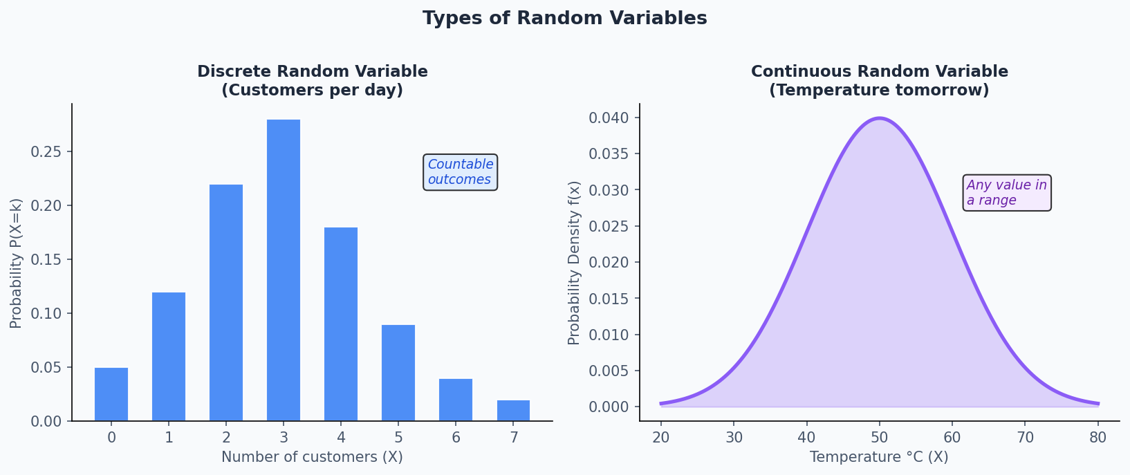
- Discrete Random Variable: takes a countable number of values.
Example: Number of customers who purchase in a day (0, 1, 2, 3 …) - Continuous Random Variable: takes any value within a range and is obtained by measuring.
Example: The exact temperature tomorrow (28.3°C, 28.31°C, 28.312°C …)
Expected Value (Mean) of a random variable X:
E(X) = Σ [xᵢ × P(xᵢ)] [for discrete random variables]
E(X) = ∫ x × f(x) dx [for continuous random variables]
The expected value is the long-run average outcome if an experiment is repeated infinitely many times. In Machine Learning, the loss function is the expected value of the prediction error over the training data.
5. Probability Distributions Every Data Scientist Must Know
A probability distribution describes how probabilities are assigned to each possible value of a random variable, the complete picture of uncertainty across all outcomes.
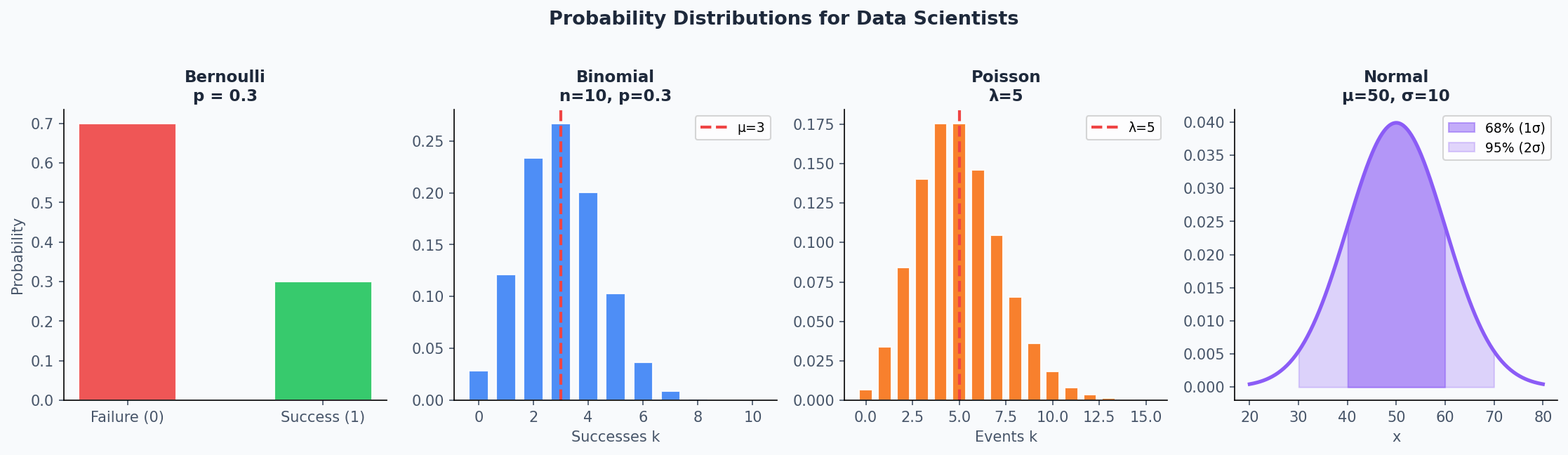
5.1 Normal Distribution (Gaussian)
The Normal Distribution is the most important in data science. It is symmetrical, bell-shaped, and fully described by two parameters: mean (μ) and standard deviation (σ).
f(x) = (1 / σ√2π) × e^(-(x-μ)²/2σ²)
The 68-95-99.7 Rule:
– 68% of data falls within 1σ of the mean
– 95% of data falls within 2σ of the mean
– 99.7% of data falls within 3σ of the mean
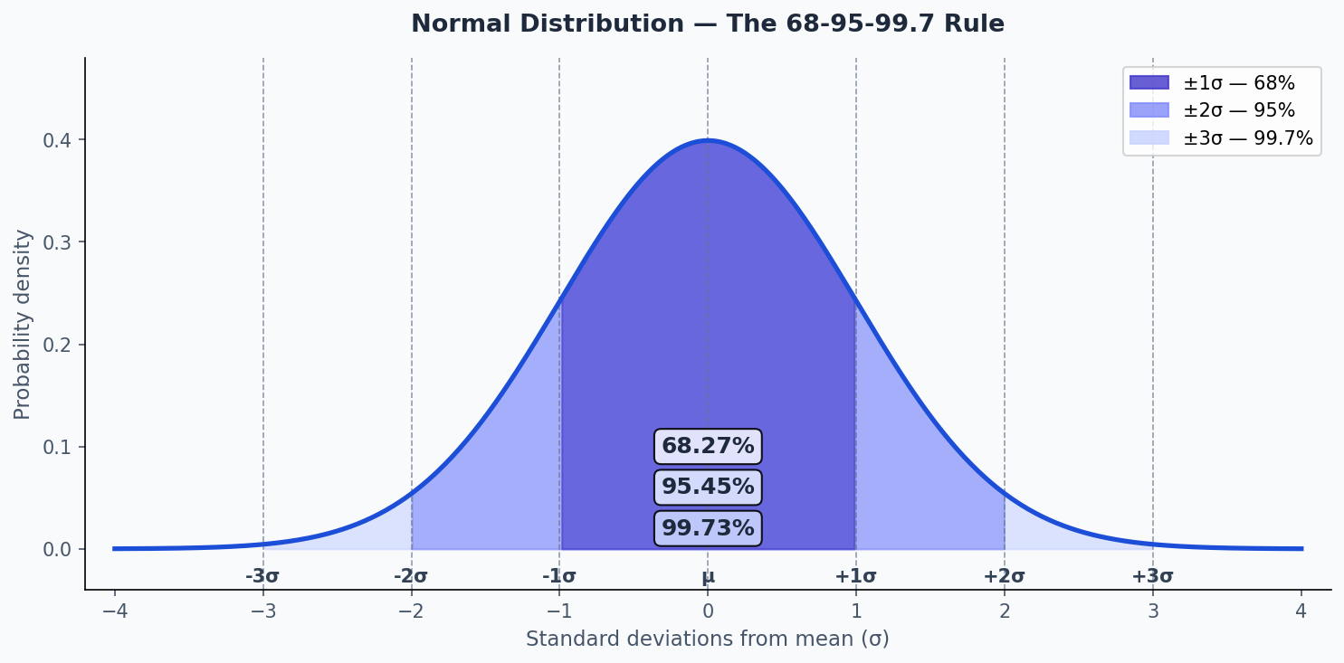
Why it matters: Many ML algorithms assume normally distributed data or residuals. Feature normalisation, anomaly detection, and confidence intervals all rely on the Normal Distribution.
5.2 Binomial Distribution
Models the number of successes in ‘n’ independent trials, where each trial has only two outcomes: success (1) or failure (0), with probability of success ‘p’.
P(X = k) = C(n,k) × pᵏ × (1-p)^(n-k)
Real-world Example: If 30% of users click a notification, what is the probability that exactly 4 out of 10 users click? That is a binomial probability problem.
5.3 Poisson Distribution
Models the number of events occurring in a fixed interval of time or space, given a known average rate λ, when events happen independently of each other.
P(X = k) = (λᵏ × e^(-λ)) / k!
Real-world Example: A server receives an average of 5 requests per second. What is the probability of receiving exactly 8 requests in the next second? That is a Poisson problem.
5.4 Bernoulli Distribution
The simplest distribution: a single trial with two outcomes: success (1) with probability p or failure (0) with probability 1−p. It is the building block of the Binomial Distribution.
P(X = 1) = p
P(X = 0) = 1 – p
Every binary classification problem in Machine Learning- spam or not spam, fraud or not fraud, churn or not churn- is fundamentally a Bernoulli random variable.
6. Probability in Python: Hands-On
You do not need to compute probability by hand as a data scientist. Python handles everything. I have uploaded a complete Jupyter Notebook on GitHub with examples. Click on the link below:
https://github.com/nidhibansal1902/Probability_for_Data_Science
D. Where You’ll Use Probability as a Data Scientist
Here are some examples where you will use probability as a data scientist.
| AI System | Probability Concept |
| Gmail Spam Filter | Bayes Theorem |
| Netflix Recommendations | Conditional Probability |
| ChatGPT | Next-word Probability |
| Self-driving Cars | Bayesian Inference |
| Medical Diagnosis | Bayes Theorem, posterior probability |
| Fraud Detection | Bernoulli + Bayes |
| Credit Risk | Logistic Probability |
| Search Engines | Ranking Probabilities |
Stay Tuned!!
Congratulations! You now understand one of the most important mathematical foundations of Data Science: Probability.
In the next article, we’ll build on these concepts by exploring Statistics, where probability helps us make informed decisions from real-world data using sampling, measures of central tendency, measures of spread, confidence intervals, and hypothesis testing.
Explore the complete series:
- Linear Algebra
- Coordinate Geometry
- Planes
- Matrices
- Calculus
- Statistics (Next)
Keep learning and keep implementing!!

