Master SQL for Data Science (With Real Examples)
After learning Python and the basics of Mathematics, it is time to learn SQL.
Most beginners skip SQL and jump straight to Machine Learning. That is a mistake, because before you build a single model, you need to access, retrieve, and understand your data. And data lives in databases. SQL is the key to accessing those databases.
In this article, you will learn why SQL is essential for every data scientist, the core commands you need to know, and how to query a real database directly inside your Jupyter Notebook using Python, no separate database server needed.
Why Do Data Scientists Need SQL?
As all data is stored in databases, data scientists need to know how to retrieve data and use it for analysis, machine learning models, and prediction.
Every company, from a startup to a Fortune 500, stores its data in databases like product data, customer data, sales data, transaction data, and all of it lives in structured tables inside a database.
SQL (Structured Query Language) is the query language used to interact with databases. Without SQL, you cannot access the data you need as a data scientist.
Here is the key distinction to keep in mind early on: SQL is a declarative programming language, not a procedural one like Python, C++, or Java. In Python, you tell the computer how to do something step by step. In SQL, you tell the database what you want, and it figures out how to retrieve it for you.
You do Not Need MySQL Workbench
Here is something most SQL tutorials do not tell you. You do not need to install MySQL Workbench or set up a separate database server to practise SQL and to access data as a data scientist.
Python has a built-in library called “SQLite3” that lets you connect to and query a database directly inside your Jupyter Notebook. SQLite3 comes pre-installed with Python with zero setup required.
This means you can practise real SQL on real data, right now, in the same environment where you already do your data science work.
How to use SQLite3 directly in Python
To use SQLite3, you need to import SQLite3 in your Jupyter Notebook and establish a connection with the database. Below is the sample code for it.
#import libraries
import sqlite3# Connect to your SQLite database
conn= sqlite3.connect(“classic_rock.db”)
print(“Database connected successfully!”)
Core SQL Commands Every Data Scientist Must Know
Level 1 — Data Retrieval Basics
These four commands answer almost any business question from a dataset:
- SELECT — which columns you want
- FROM — which table to get them from
- WHERE — filter rows by a condition
- COUNT— gives a numerical count of rows
- DISTINCT— gives unique values present in a given column
- GROUP BY — aggregate data into groups
Level 2 — Advanced Filtering and Sorting
SQL commands for advanced filtering and sorting in database tables.
- HAVING — filter groups after GROUP BY
- ORDER BY — sort your results (by default in ascending order)
- LIMIT — returned top N or bottom N number of rows
- OFFSET — skip a certain number of rows
The order of query execution in SQL is:
FROM→ WHERE → GROUP BY → HAVING → ORDER BY
Level 3 — Combining Tables
SQL Command used to join two or more tables, as in real scenarios, data Scientists need to merge the tables often to create meaningful insights for business.
- JOIN and ON— used to merge two tables and retrieve data from them.
There are four types of JOIN: INNER, LEFT, RIGHT, and FULL OUTER. INNER JOIN is the most commonly used in data science work.
Hands-On: Query a Real Database in Jupyter Notebook
For this tutorial, we will use the “Classic Rock Songs” database with the name classic_rock.db, a real dataset containing 1,650 classic rock songs, 37,673 radio play records across multiple radio stations, artist play counts, release years, and timestamps.
You can download the database and the complete Jupyter Notebook from the GitHub link:
https://github.com/nidhibansal1902/Master-SQL-for-Data-Science
Step 1: Connect to the Database
#import libraries
import sqlite3
import pandas as pd# Connect to the SQLite database
conn = sqlite3.connect(‘classic_rock.db’)
print(“Database Connected successfully!”)
Step 2: Explore the Tables
# Execute the query to fetch tables
query = “SELECT name FROM sqlite_master WHERE type=’table’;”# Fetch and clean up the results
tables = pd.read_sql_query(query, conn)
print(“Tables in the database:”)
print(tables)Output>>
Tables in the database:
name
0 rock_songs
1 rock_plays
This database has two tables — `rock_songs` (song and artist information) and `rock_plays` (radio station play records).
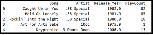
Step 3: Retrieve Your First Data using SELECT
# Get first 5 songs
query = “SELECT Song, Artist, Release_Year, PlayCount FROM rock_songs LIMIT 5;”
df = pd.read_sql_query(query, conn)
print(df)Output>>
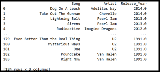
Step 4: Filter Your Data using WHERE
# Find all songs released after 1990
query = “SELECT Song, Artist, Release_Year FROM rock_songs WHERE Release_Year > 1990 ORDER BY Release_Year DESC; ”
df = pd.read_sql_query(query, conn)
print(df)Output>>
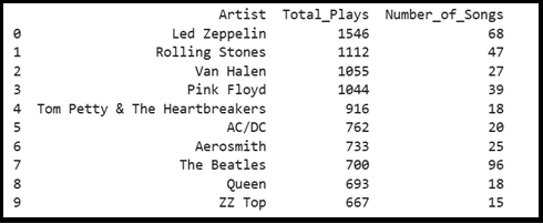
Step 5: Aggregate and Summarise using GROUP BY
# Top 10 most played artists
query = “””SELECT Artist,
SUM(PlayCount) AS Total_Plays,
COUNT(*) AS Number_of_Songs
FROM rock_songs
GROUP BY Artist
ORDER BY Total_Plays DESC
LIMIT 10;
“””
df = pd.read_sql_query(query, conn)
print(df)Output >>
Download the complete Jupyter Notebook with many more example queries from GitHub.
Complete Jupyter Notebook uploaded on GitHub
I have uploaded the complete SQL Jupyter Notebook and database ‘classic_rock.db’ to GitHub. Click here to access the notebook and download the database from GitHub, and place both in the same folder.
Stay Tuned!!
For system setup for data science with Python, click on the link below.
Keep learning and keep implementing!!

